Download this example as a Jupyter notebook.
Nbsphinx example#
This example renders a Jupyter notebook using the nbsphinx extension.
Plot a simple sphere using PyVista.#
[1]:
import pyvista as pv

pv.set_jupyter_backend("html")

sphere = pv.Sphere()
sphere.plot()
[2]:
plotter = pv.Plotter(notebook=True)
plotter.add_mesh(sphere, color="white", show_edges=True)
plotter.title = "3D Sphere Visualization"
plotter.show()
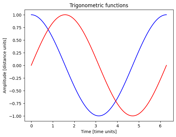
Figures with Matplotlib#
This example shows how to render a figure using Matplotlib.
[3]:
import matplotlib.pyplot as plt
import numpy as np

time = np.linspace(0, 2 * np.pi, 100)

fig, ax = plt.subplots()
ax.plot(time, np.cos(time), color="blue", label=r"$\cos{(t)}$")
ax.plot(time, np.sin(time), color="red", label=r"$\sin{(t)}$")

ax.set_xlabel("Time [time units]")
ax.set_ylabel("Amplitude [distance units]")
ax.set_title("Trigonometric functions")

plt.show()
Figures with Plotly#
This example shows how to render a figure using Matplotlib.
[4]:
import plotly
import plotly.graph_objs as go

time = np.linspace(0, 2 * np.pi, 100)

cos_trace = go.Scatter(x=time, y=np.cos(time), mode="lines", name="cos(t)")
sin_trace = go.Scatter(x=time, y=np.sin(time), mode="lines", name="sin(t)")

fig = go.Figure(data=[cos_trace, sin_trace])
plotly.io.show(fig)
Data type cannot be displayed: application/vnd.plotly.v1+json
Render equations using the IPython math module.#
[5]:
from IPython.display import Math, display

# LaTeX formatted equation
equation = r"\int\limits_{-\infty}^\infty f(x) \delta(x - x_0) \, dx = f(x_0)"
# Display the equation
display(Math(equation))
$\displaystyle \int\limits_{-\infty}^\infty f(x) \delta(x - x_0) \, dx = f(x_0)$
[6]:
from IPython.display import Latex

Latex(r"This is a \LaTeX{} equation: $a^2 + b^2 = c^2$")
[6]:
This is a \LaTeX{} equation: $a^2 + b^2 = c^2$
Render a table in markdown.#
This is an example to render the table inside the notebook
A |
B |
A and B |
|---|---|---|
False |
False |
False |
True |
False |
False |
False |
True |
False |
True |
True |
True |
Render a data frame#
[7]:
import pandas as pd

# Create a dictionary of data
data = {
    "A": [True, False, True, False],
    "B": [False, True, False, True],
    "C": [True, True, False, False],
}

# Create DataFrame from the dictionary
df = pd.DataFrame(data)

# Display the DataFrame
df.head()
[7]:
| A | B | C | |
|---|---|---|---|
| 0 | True | False | True |
| 1 | False | True | True |
| 2 | True | False | False |
| 3 | False | True | False |